A very short introduction to Non-Linear Dynamics

Alvaro Aguirre - August 2020

During my time at the LSE I studied Non-Linear Dynamics and chaotic systems, and found it fascinating. We normally think in linear terms, which is a huge problem because the world is highly non-linear. So in this short post I want to give you a very brief and basic introduction to chaos theory.

“It used to be thought that the events that changed the world were things like big bombs, maniac politicians, huge earthquakes, or vast population movements, but it has now been realized that this is a very old-fashioned view held by people totally out of touch with modern thought. The things that change the world, according to Chaos theory, are the tiny things. A butterfly flaps its wings in the Amazonian jungle, and subsequently a storm ravages half of Europe.” — Terry Pratchett and Neil Gaiman

In a non-linear system, a change in output is not proportional to a change in inputs. And this very simple characteristic makes studying the dynamics of this type of systems very fun. To give you a first taste of the power of non-linearities, consider the next two options:

1) I will give you 10 million dollars each day for the next 100 days.
2) I will give you only one cent today, but every day for the next 100 days, the amount of money you have will double.

If you choose option 1, which clearly sounds more appealing at first glance, you will end up with the modest sum one billion dollars. Not bad… But if you had chosen option 2, you would have ended up with 6.33e27 dollars, which is roughly about 7 trillion times the GDP of the world.

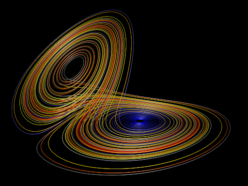
But what I want to tell you about non-linear systems goes beyond the difference between linear and exponential, which you probably already know. It is how sensitive a non-linear system can be to its initial conditions. The quote above mentions the famous “butterfly effect”. The metaphors tells us that a tiny change in the initial condition of a system, which for our linear minds should make no difference at all, can actually make a huge difference in the dynamics of the system over time. The graph above, which resembles a butterfly’s wings, is actually one of Ed Lorenz’ strange attractors. He is considered to be the father of Chaos Theory.

Perhaps the best way to illustrate the beauty of non-linear dynamics is with a graphical example. So let’s consider a system that evolves according to the following rule:
\(x_{n+1} = a x_n (1-x_n)\)
This is the famous Logistic Map. The system is initialized with an initial condition, which we shall call \(x_0\), and a given parameter value for \(a\). Then we just let the system “run”. At every iteration, we will get a new value of \(x\), which will then become the “input” in the next iteration, and so on…

So how will this system behave over time? I have to give you the classical economist answer: it depends! And boy does it depend… We will see that the dynamics of the system can be absolutely different depending on the parameter value we set. Here is where our linear minds come in and say “I’m pretty sure tiny changes in a won’t make much of a difference”, or that is at least what my linear mind thought before tackling this problem. Let’s see what happens.

The next graph shows the dynamics of the system for different values of the parameter \(a\). Each point in the graph is the state of the system after running for a long time (>=1024 iterations), where the initial condition x0 has been drawn from a Uniform(0,1) distribution.

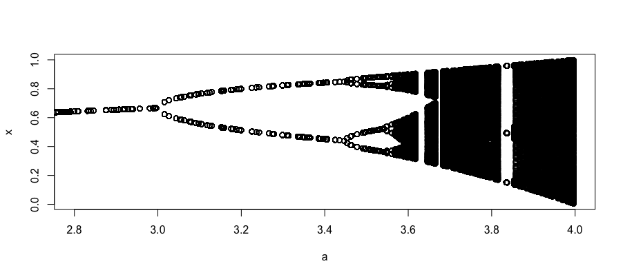
So how do we interpret this? Consider the value \(a = 2.8\). We see there is only one point as the image, at around \(x = 0.64\). That means that the dynamics of the Logistic Map for \(a = 2.8\) is just a single attractor. So, over time, the system reachs a point and stays there. What about a value of \(a = 3.2\)? We then see that it maps to two values of \(x\), meaning that for such value of the parameter, the state will have two attractors and will be stuck looping between those two points forever. As you can see, the behavior of the system over time is absolutely different depending on the value of \(a\). In particular, we can see a bifurcation diagram. For small values of \(a\), we have a single value of \(x\), then, for some value of \(a\), it splits into two, after a while, it splits again into four, after another while (but shorter this time), it splits into eight, then sixteen, and shortly we cannot keep track anymore, it’s chaotic! For a value like \(a = 4\), we have no idea of what’s going on. The system keeps moving around between 0 and 1 with no apparent pattern.

BUT, that is not the cool part. You have probably already noticed something very odd in the graph. What happens at around \(a = 3.84\)!? A three-period loop? In the middle of that messy chaotic system? There’s something weird going on there. We had a well-behaved bifurcation diagram, and for some reason it just condenses into a period-three loop for some values of \(a\). Let’s zoom into this region to see what is happening:

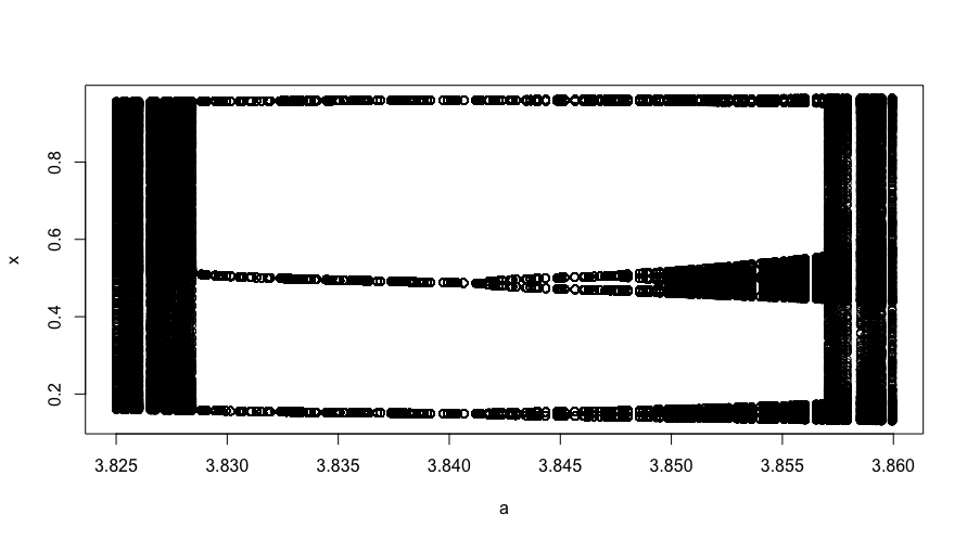
Ok so zooming in, it turns out it was not a single point of \(a\), but there is an entire bifurcating system within our bigger system! The system is jumping around, behaving chaotically, and then it immediately condenses into three points. It is not a smooth reduction, but a sharp one. For some value of \(a\), the dynamics drastically change and the system seems to behave “nicely”, with \(x\) jumping between just three values. With further increases in \(a\), we see how chaos re-emerges in our system, with new bifurcations, but then again, there is a sudden change at around \(a = 3.857\).

Let’s zoom in once again:

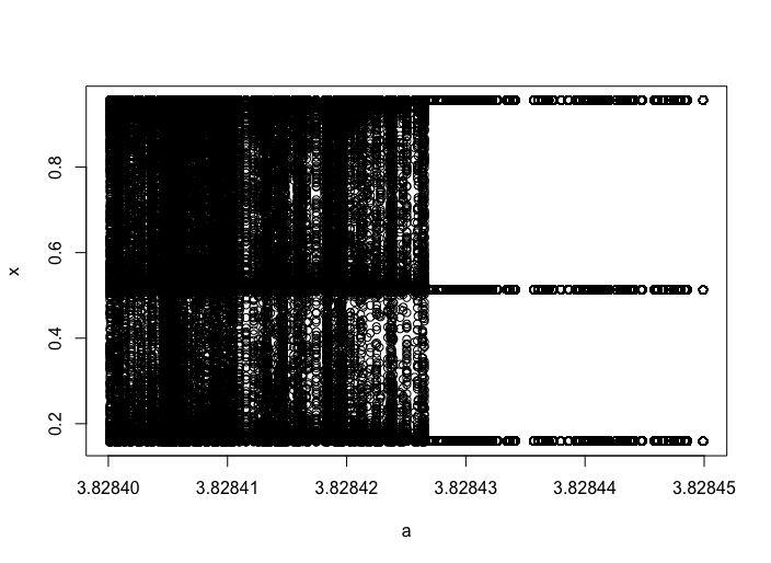
Here we can see a close-up on how the system condenses into a period-three loop. We are already looking at differences of less than a thousandth of \(a\). Imagine you are a researcher conducting an experiment, and you have to set up the value of the parameter \(a\), and you are not sure if you should pick 3.82842 or 3.82843. Of course the output of any model changes with changes in the parameters, but here we are talking about a drastic change in the behavior of the system (from chaotic to period-three). This is a case where a rounding error can have a huge impact on your results. You might think Oh it’s all good, I work with a very fancy computer, no rounding errors. Digital computers, by definition, will always make tiny rounding errors (a study done at UCL about this can be found here). If you don’t believe me, try this simple addition on any programming language in your computer: 0.1 + 0.2 - 0.3.

Mathematically, of course, this is zero. I just ran this on Python on my Terminal, surprise: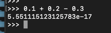

Yes, this is a very, very, very small number. But as I just showed you above, in some systems, even the smallest difference can have a drastic effect.

Do you want to learn more about this? This video is a fantastic explanation that dives deeper into what we have discussed.